Evaluating Jim Hansen’s 1988 Climate Forecast
May 29th, 2006Posted by: Roger Pielke, Jr.
A lot of attention has been paid by both sides of the climate debate to a prediction made in 1988 before Congress by NASA scientist James Hansen. Today this forecast is the subject of an op-ed by Paul Krugman in the New York Times in which he accuses a prominent climate skeptic of scientific fraud. For some time I have been interested in various claims about Jim Hansen’s forecast because I am interested in prediction and its use/misuse in policy and politics. But what has been missing to date is a rigorous evaluation of Hansen’s forecast. Here is an initial effort to bring a bit more rigor to such an evaluation. The numbers below are not the last word, may contain errors, and are intended to open a discussion on this subject.
Hansen’s 1988 prediction was based on an analysis presented in this paper:
Hansen, J., I. Fung, A. Lacis, D. Rind, S. Lebedeff, R. Ruedy, G. Russell, and P. Stone 1988. Global climate changes as forecast by Goddard Institute for Space Studies three-dimensional model. J. Geophys. Res. 93, 9341-9364. (Abstract)
The paper generated future climate predictions based on three scenarios, described in the abstract as follows:
Scenario A assumes continued exponential trace gas growth, scenario B assumes a reduced linear linear growth of trace gases, and scenario C assumes a rapid curtailment of trace gas emissions such that the net climate forcing ceases to increase after the year 2000.
In this PDF, Jim Hansen provided an image of the prediction for the three scenarios with an overlay of the actual temperature increase in a response to Michael Crichton. I have reproduced the figure immediately below.
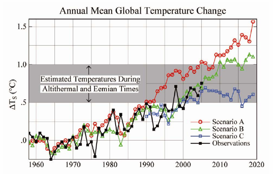
The observations (black) are very closely matched to Scenario B. Consequently, Jim Hansen claimed, “the real world has followed a course closest to that of Scenario B” (PDF). But is this correct? It appears that Jim Hansen may have gotten the right answer on temperature for the wrong reasons because his assumptions about emissions paths were not accurate. Further, Scenario B with the best match to temperature is the most inaccurate with respect to emissions projections.
The three scenarios used by Jim Hansen were based on assumptions about how society would produce emissions forward from 1988. Key assumptions were made for methane (CH4), Nitrous Oxide (N2O), and Carbon Dioxide (CO2) – For scenarios A and B in developing and developed countries, and for the global total in the case of Scenario C. Here are the assumptions from Hansen’s 1988 paper for growth rates in CH4, N2O, and CO2:
Scenario A
CH4 0.5%
N2O 0.25%
CO2 3% developing, 1% developed
Scenario B
CH4 0.25%
N2O 0.25%
CO2 2% developing, 0% developed
Scenario C
CH4 0.0%
N2O 0.25%
CO2 1.6 ppm increase annually
In order to evaluate whether these assumptions played out as projected in the three scenarios I consulted online databases with estimates of increases in CH4, N2O, and CO2.
I found CH4 data for 1990-2005 in an EPA report (PDF) in Appendix A-II.
I found N2O data for 1990-2005 in the same EPA report (PDF) in Appendix A-3.
I found CO2 data from the UN FCCC in a recent report (PDF) , for Annex I countries in table II-3 for 1990-2003.
I found global CO2 levels for 1990-2005 in the U.S. government database.
I used this data to compare growth rates in CH4, N2O, and CO2 to Jim Hansen’s 3 scenarios from 1988. Here is what I found:
Actual Rate of Increase
CH4 0.46%
N2O 0.95%
CO2 -0.52% (Annex 1 Countries 1990-2003)
CO2 >4.5% (Non-Annex 1 Countries 1990-2003)
CO2 1.5 PPM (1990-2005)
Comparison with Scenarios
Most Accurate CH4 Assumption = Scenario A
Most Accurate N2O Assumption = each
Most Accurate CO2 Assumption = Scenario C
In none of the three emissions assumptions did Scenario B contain the most accurate emissions assumptions. From this initial evaluation, it seems that to the extent that Jim Hansen’s Scenario B has accurately anticipated global temperature increases since 1988, it has done so based on inaccurate assumptions about emissions paths. Perhaps the errors cancel out, but an accurate prediction based on inaccurate assumptions should give some pause to using those same assumptions into the future. I am not sure which Scenario would be evaluated as the most accurate, but given the importance of CO2 as a greenhouse gas, I’d lean toward Scenario C. None of this is to doubt that global temperature has increased or will continue to increase as projected by the IPCC.
The usual caveats apply: This analysis provides no support for anyone who would cherry pick one scenario over another to evaluate their accuracy (as Paul Krugman has accused Patrick Michaels and Michael Crichton of doing). Nor does this analysis provide any reason not to support the importance of action on climate policy.
What it does, however, is raise questions about how scientists are treated differently in the public by other scientists and the media, and importantly, how some instances of policy-relevant science are framed critically and other instances are framed quite positively. Take William Gray for example who spent decades warning about a coming increase in hurricane activity, who was proven correct when activity increased, only to be frequently excoriated by his peers for his views on global warming. On hurricanes, Gray may have been right for the wrong reasons, but he was nonetheless right in his warning. Hansen on the other hand, is feted by his peers and the media yet just like Bill Gray may have been right for the wrong reasons.
May 29th, 2006 at 10:28 pm
Roger-
I think you have an oversimplistic view of this. Bill Gray is excoriated in public, rightfully in my opinion, because he’s essentially accused the entire scientific community of fraud … and for no other reason that I can figure out other than he didn’t get the funding he feels he deserves. As a scientist, he knows that the type of conspiracy theories he’s suggesting simply cannot actually occur. This has led to a real loss of respect within the community for him. [did you see the paper he submitted to the AMS tropical meteorology conference? it actually had a quote from Inhofe in it!!! how can he expect to be taken seriously?]
Jim Hansen, however, remains a well-respected scientist. I think that most alert people also recognize that Hansen has become an advocate, so evaluating him is somewhat problematic — some of the love of Hansen results from the fact that many scientists agree with his advocacy positions, and some of it results from the fact that he “sticks i to the man,” e.g., the whole Deutsch affair.
Also, I loved Hansen’s single MMMBop. Catchy!
Regards
May 29th, 2006 at 10:39 pm
Roger,
To evaluate scenario B, you are asking us to compare this reality:
CO2 -0.52% (Annex 1 Countries 1990-2003)
CO2 >4.5% (Non-Annex 1 Countries 1990-2003)
CO2 1.5 PPM (1990-2005)
to this projection:
CO2 2% developing, 0% developed
Can someone do the conversion? Ideally from “CO2 2% developing, 0% developed” to ppm/yr
May 30th, 2006 at 12:03 am
Roger,
This seems rather petty. Rather than looking at the details of every different GHG, it would be more meaningful to look at the overall forcing and how the climate responded to it. After all, predicting future CO2 (etc) levels is hardly in the domain of the climate scientists – but what we can tell you about is the relationship between emissions and climate change (with at least some degree of accuracy, as Hansen has shown). I’ve no doubt that if you were to re-run this model with observed GHG changes (and eg pinatubo in the right place), the output would match observations very well indeed.
Of course, it turns out that predicting the medium-term temperature change is a pretty easy thing to do – but we only know that through the work of climate scientists in understanding both how the climate responds to forcing, and how the anthropogenic forcing dominates natural effects.
May 30th, 2006 at 2:57 am
B and C look rather similar up to now. It seems odd to worry about the differences.
May 30th, 2006 at 4:44 am
It would be rather interesting if his 1988 prediction did turn out to be correct, given that it was made using a low-resolution model with a sensitivity to doubling CO2 of 5.1, a slab ocean and (I believe) no anthropogenic sulphates.
You don’t need to compare with observations to know that the model had deficiences. The deficiences were known at the time, but the model did allow some broader conclusions, which is what I think Hansen was primarily driving at.
The key things that Hansen predicted (all of which turned out to be true) were that: 1. temps would keep rising as GHG concs increased – not year on year, but with an average trend. 2. The trend rate of rise is dependent on emissions, but under reasonable assumptions is meaningful and will soon (from 1988’s perspective) be detectable. 3. That the rate of rise is tempered by ocean heat uptake. 4. Stopping emissions will not imediately stop temp rise (ocean heat uptake again).
btw, if anyone want to run Hansen’s model with observed forcing (no anthro sulphates or volcanoes), they can at http://www.edgcm.org
May 30th, 2006 at 4:53 am
BTW, the GISS model II has a sensitivity of 5.1 if you run it to equilibrium, and 4.2 if you run it for 25 years (as was done in the original 1983 paper, hence Hansen’s statement of a 4.2 sensitivity).
BTW 2. Where did you get your figures for the scenarios? I though B and C were the same, except that in C emissions were curtailed in the yr 2000. See http://www.giss.nasa.gov/edu/gwdebate/
May 30th, 2006 at 5:41 am
unfortunately I can’t read the Op-Ed because I don’t subscribe to the NYT.
WHat I am interested in, if someone can tell me is why secnario B is considered the closest to the 1988-2003 evolution?
JUst looking at the chart leaves one thinking that B and C could be indistinguishable from a statistical perspective from one another, let alone from the post 1988 time series.
What is also confusing is the basis for the assumption set. For A and C we have disgaggregated growth rates, for C it is a ppm global figure. These need to be standardised.
I would suggest that the best you could probably say about this with any reliable precision is that the evolution proved to be at the bottom end of the range of ex ante forecasts and the exogenous variables came in towards the bottom of the range of scenarios.
May 30th, 2006 at 6:03 am
Andrew-
I largely agree with your comment. Though it would be nice to see a bit more nuance in evaluations of Bill Gray — it is quite possible that he was on target on his decadal hurricane forecast but is out to lunch on his global warming views.
MMMBop? .. I’m worried (but not as much as by the fact that I get the allusion;-)
Thanks!
May 30th, 2006 at 6:10 am
James-
I remain baffled why you think a post like this must be responded to by calling me “petty.” James Hansen presented the 3 scenarios for the various GHG emissions in a peer reviewed paper. It seems entirely appropriate to subsequently ask — how did things turn out?
As such, your comment is more appropriately directed to Jim Hansen, who decided to project individual GHG emissions in his 1988 paper and continue to use that framework as the basis for presenting his work to policy makers and the public.
Another useful exercise would be to take a linear projection of temperature increase from 1988 and compare acutals and the 3 scenarios to the naive extrapolation to assess whether the forecast had any skill. Perhaps that also would demonstrate pettiness?
Thanks.
May 30th, 2006 at 7:30 am
Roger,
Can you calculate the GHG growth rates for the different scenarios (and observations) in terms of CO2 equivalents? Which scenario is closest in this regard? Answering these questions might be a better way of evaluating model skill, compared with observations.
Also, I tend to agree with Dr. Connelly, that model runs B and C appear very similar up to 2005.
May 30th, 2006 at 8:14 am
James-
Agreed. Perhaps this is how Hansen should have framed his original analysis.
If B and C are indistinguishable, then does Jim Hansen exceed the bounds of what can be conclusively asserted when he asserts that the “real world has followed a course closest to Scenario B”?
May 30th, 2006 at 8:16 am
Roger,
On a different subject, I think Krugman’s op-ed raises an interesting question that has been visited frequently on this site: the use and misuse of science to advance a political agenda.
First, let me say, that I tend to agree with your position that scientists should be careful in public discussions of global warming to avoid playing the role of issue advocate (or, they should at least be aware that taking a strong policy position poses it’s risks). Of course, there seems to remain some disagreement over where, exactly, the line exists between defending science (and scientists) and advocating specific policy solutions. I thnk that Prometheus has provided a very useful forum for helping to define this line.
But what about politicians? If I am not mistaken, you have argued that Senator Inhofe’s public statements on the Senate floor and on TV that, “global warming is a hoax” are not entirely inappropriate because he is merely using inflated rhetoric to make a political point. Also, his calling of witnesses like Crichton before a Senate Committee to argue against the existence of a global warming threat is, I think you have said, just what politicians (and lawyers) do. They marshal a suite of (cherry picked) facts in support of an argument and they oversell that argument to advance their cause. (If I have misrepresented your position in any way, please set me straight).
So, if Inhofe’s portrayal of reality — in his capacity as the Chairman of the Senate committee for the Environment and Public Works — is not to be harshly condemned by all, then why is it not a double standard to expect Al Gore (or any other advocacy agent or politician) to stay strictly within the bounds of what is scientifically proven, when making their case for public policy aimed at slowing the rate of GHG emissions? For example, your comment at RealClimate earlier this month seemed to be condemning Gore for making “scientifically indefensible” arguments in support of his cause. Perhaps he was doing this… I have not yet seen the movie. But if he was, how is that different from what Inhofe does all the time?
So, I am wondering if there are different standards for politicians, columnists and scientists in this world of marshaling scientific facts in support of a political cause? If so, what are those standards? Finally, do you think that Krugman is onto something when he writes: “And it’s a warning for Mr. Gore and others who hope to turn global warming into a real political issue: you’re going to have to get tougher, because the other side doesn’t play by any known rules?”
Many thanks for your time.
May 30th, 2006 at 8:36 am
James (Bradbury)-
Thanks for these thoughtful comments and questions.
You are certainly correct that Gore’s invocation of hurricanes and extreme events is of course a tactic of political advocacy. The issue that I have is that Gore’s policy recommendation — that we use greenhouse gas mitigation to address hurricane impacts — simply can’t work as advertised. Similalry, Senator Inhofe’s absurd conclusion that global warming is a hoax, and presumably that we should do nothing in response, is also a recipie for poor policy.
The difference, as I see it, is that while Senator Inhofe is roundly criticized in the community for arguing for policies that will be unlikely to have their intended effects, Al Gore gets a complete free pass from the community — even though his policy recommendations are just as ineffectual as those proposed by Sen. Inhofe! Of late, I have focused on Al Gore’s portrayal of hurricanes because it is an area in which I am doing primary policy research.
So I am less concerned with Inhofe’s and Gore’s “portrayal of reality” than with the practical implications of such portrayals for actual policy action.
So the issue is much less about “science” per se, than it is about how we evaluate the potential efficacy of alternative policy options that politicians bring to the public. Such evaluations of course can and should be done scientifically but they are focused on policy options, not simply scientific “truths” (see discussions of the linear model for how people define “science” differently.)
If this doesn’t get to what you were asking, please ask again.
Thanks!
May 30th, 2006 at 8:40 am
Roger,
“…does Jim Hansen exceed the bounds of what can be conclusively asserted when he asserts that the ‘real world has followed a course closest to Scenario B’”
I see your point, and perhaps he has exceeded the bounds of what can be “conclusively” asserted. However, I don’t think that Hansen has ever suggested that this assertion was “conclusive.” He also never said that the real world has turned out nothing like run C, has he?
May 30th, 2006 at 9:02 am
James (B.)- Thanks, but a similar argument (referring to Krugman’s allegations about Pat Michaels) would be that Pat Michaels never said that Hansen’s prediction was not closer to Scenario B or C when he cherrypicked Scenario A as a comparison. I’d reject such a claim. Shouldn’t we treat errors of omission equally no matter who is making them?
Perhaps we should just agree that Hansen would be well-served in the future to simply point out that:
a) Temperature has followed the curves of B and C
b) However, neither scenario provides a good representation of actual emissions paths underlying the scenarios
c) But perhaps they (by accident) B and C got GHG forcing about right
Thanks!
May 30th, 2006 at 9:04 am
Roger,
Thanks for your response.
“So I am less concerned with Inhofe’s and Gore’s “portrayal of reality” than with the practical implications of such portrayals for actual policy action.”
That seems reasonable to me.
Although, as you may recall, I tend to get more upset by Inhofe because 1) of my own policy preferences and 2) the Senator from OK is in a very powerful position when it comes to actually making public policy, not just proposing it (while Al Gore is not). Also, Inhofe took an oath to serve the public, but he chooses to use his influential committee to host talk-show-style panels with fiction writers posing as scientists. This puts off a strong scent of contempt for an honest debate and so I think it does more than distort reality… it undermines public trust in the democratic process and good governance.
Sorry if this strays too far off topic. Thanks again for your response.
Best, James
May 30th, 2006 at 9:55 am
Tom-
In response to you BTW2:
The emissions rates I cite are from table 3 of this paper:
Hansen, J., Mki. Sato, J. Glascoe, and R. Ruedy 1998. A common sense climate index: Is climate changing noticeably?. Proc. Natl. Acad. Sci. 95, 4113-4120.
http://pubs.giss.nasa.gov/docs/1998/1998_Hansen_etal_1.pdf
Take a close look at Figure 5C which is a more sophistocated analysis than that presented here. Through 1998 it actually suggests that scenario C was the more accurate of the three.
In that paper, Hansen wrote:
“The large interannual variability of even global mean temperature makes it difficult to draw inferences about model validity based on only a decade of observations. But, at least so far, the real world is behaving more like the model driven by scenarios B and C, rather than the model driven by scenario A.”
May 30th, 2006 at 10:00 am
Roger,
Regarding your first point. I think the figure basically speaks for itself… especially when results from all of the model runs are left on the figure so that the viewer can make a judgment. Michaels, on the other hand, had to *erase* two of the runs to make his point seem valid.
I will grant you that one of Krugman’s points is misleading: “The original paper showed a range of possibilities, and the actual rise in temperature has fallen squarely in the middle of that range.” But Hansen never said this.
Also, regarding you conclusions:
“a) Temperature has followed the curves of B and C”
OK, fair enough.
“b) However, neither scenario provides a good representation of actual emissions paths underlying the scenarios.”
In the context of this discussion of model skill with respect to GHG forcing, I think that this point is meaningless without calculating the CO2 equivalents.
“c) But perhaps they (by accident) B and C got GHG forcing about right”
Again, I think you need to calculate the CO2 equivalents to say this with any accuracy.
Thanks, James
May 30th, 2006 at 10:18 am
James-
Our comments may have crossed in the ether, but my response to Tom addresses your points. See Figure 5C in this paper:
Hansen, J., Mki. Sato, J. Glascoe, and R. Ruedy 1998. A common sense climate index: Is climate changing noticeably?. Proc. Natl. Acad. Sci. 95, 4113-4120.
http://pubs.giss.nasa.gov/docs/1998/1998_Hansen_etal_1.pdf
This goes through 1996 (apparently?). I am unaware of any update to this figure.
As far as your point b), I can’t imagine how one can conclude that estimates of future emissions are “irrelevant” since such estimates are the basis for predictions of the type Hansen has offered since 1988.
Thanks.
May 30th, 2006 at 10:54 am
Roger,
Thanks, that link helps. From figure 5 and the text, it looks like the actual emissions pathway has been in between B and C of the original projections. So, the fact that observed temperatures have tracked within the range of model runs B and C suggests that Hansen’s original 1988 forecasts were very good, no? Of course, an updated version of the combined forcings through 2005 would be useful.
My earlier point (b) was just that your original method of skill-scoring the projected emissions pathways — by CH4, N2O and CO2 separately — may not be as “meaningful” as if the GHG emissions pathways (A, B, & C vs. observed) were presented in CO2 equivalents (CO2E), or in terms of total W/m^2 forcing (as done in Figure 5 of Hansen et al., 1998). I didn’t use the word “irrelevant.” Misunderstanding…
Best, james
May 30th, 2006 at 11:03 am
James- Thanks. I understand your (b) point better.
As far as emissions pathway, saying that it lies between Scenarios B and C seems incorrect. hansen writes,
“Fig. 5A reveals that the “actual” greenhouse gas forcing falls near or just below scenario C.”
Thanks!
May 30th, 2006 at 1:28 pm
The CO2 forcings in question really do not start to diverge until around 2000, when scenario C levels off with regard to CO2 emissions, so it is really not valid to say that “Hansen is right for the wrong reason” based on data through 1998 (fig 5 of the 1998 paper by hansen)
not only that, The CRITICAL thing about scenario C (as hansen points out) is that it assumes the CO2 level LEVELS off in 2000,
(“specifically greenhouse gases were assumed to stop increasing after 2000″ — JH)
http://www.columbia.edu/~jeh1/hansen_re-crichton.pdf
which is CLEARLY NOT what has happened:
annual mean groth rate
2000 1.78
2001 1.60
2002 2.55
2003 2.31
2004 1.54
2005 2.53
(which average to 2.05 ppm yearly increase over the years 2000-2005, by the way)
http://www.cmdl.noaa.gov/ccgg/trends/
That certainly coems as no surprsie to Hansen. He said that this scenario (based on the assumption of a “drastic curtailment of emissions”) was probably unrealistic to begin with. Hansen is not about the business of emissions predictions, at any rate, which is why he provided different senarios in the first place (a point that seems to elude some critics of the IPCC to this day).
Furthermore, whether any given emission scenario actually matched reality is important ONLY from the standpoint of evaluating the predicted temperatures vs actual.
And for that purpsoe, what is really important is not the overall average (of yearly increase in CO2 concentration) over a time span of several years (which actually comes out about 1.71ppm for the span between 1988-2005) but the TREND, which matches scenario B more closely than scenario C (because of the leveling off assumption for scenario B referred to above)
The upshot is that the claim that the CO2 emissions matched scenario C most closely is simply NOT correct.
That much CAN be said EVEN without seeing Hansen’s actual CO2 forcing numbers for the years between 1998 and the present for scenarios A and B.
But without seeing ALL of Hansen’s CO2 forcing numbers for years past 1998 to present I would not conclude anything further — specifically in regard to how closely scenario has B matched reality since 1998.
May 30th, 2006 at 2:26 pm
Given
1) Hansen’s assumptions:
Scenario A assumes continued exponential trace gas growth, scenario B assumes a reduced linear linear growth of trace gases, and scenario C assumes a rapid curtailment of trace gas emissions such that the net climate forcing ceases to increase after the year 2000.”
and
2) the mean annual CO2 increases — particularly AFTER 2000 when scenario C assumed the annula increases would CEASE and the trend is CLEARLY still in the postive direction! ( The trend is much more important than averages but for the years 2000-2005, CO2 increased on average by 2.0ppm per year. The slight acceleration in increase might just be “scatter about the mean” of the longer period, but the CO2 level would still seem to be increasing linearly, at a minimum)
http://www.cmdl.noaa.gov/ccgg/trends/
Given 1 and 2 above, it is a bit much (to say the least) to conclude that the
“Most Accurate CO2 Assumption = Scenario C”
May 30th, 2006 at 5:23 pm
Coby- (Comment way above) Your comment got caught in the TypeKey which is proving a pain (but which is working wonders on spam!)
Annex I is a good proxy for developed countries and hansen has the sign wrong.
Note non-Annex I has a typo, should be 0.45%, also off by a large factor. See my subsequent post on this subject for an update.
Thanks!