Atlantic SSTs vs, U.S. Hurricane Damage, Part 4
October 25th, 2006Posted by: Roger Pielke, Jr.
I am happy to report that after follow-up by Jim Elsner, I have been able to come close to replicating his results. However, the replication does not add much support to the hypothesis that Atlantic SSTs are related to normalized U.S. hurricane damage. Here is why.
First, in his paper (properly cited as Jagger et al., here in PDF) Elsner reports that their analysis was “able to explain 13% of the variation in the logarithm of loss values exceeding $100 mn using an ordinary least squares regression model.” Their analysis focused on insured losses and ours is on total losses. Their analysis is in 2000 US dollars and ours in 2005 US dollars. Because insured damages are roughly half the total economic losses, and inflation, wealth, population increase by about 5-7% per year, it makes sense to use a cut-off of $250 million for our dataset rather than $100 million – thanks to the reader who made this observation. (This has the effect of eliminating about 70% of the data, an important point which I will return to later, but for now we are simply replicating the earlier results). With the dataset parsed in this fashion we get the following results.
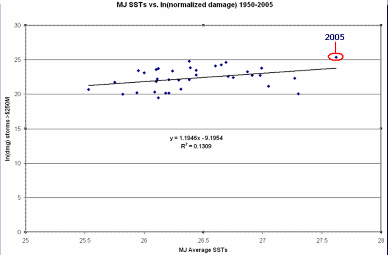
You can see that just as is reported in Jagger et al.’s paper, this result also shows an r^2 of 0.13 and I get a p value of 0.03, so the results are significant. I am satisfied that we have faithfully replicated his analysis! But what happens when one looks at the relationship from 1950-2004? The following graph shows this result.
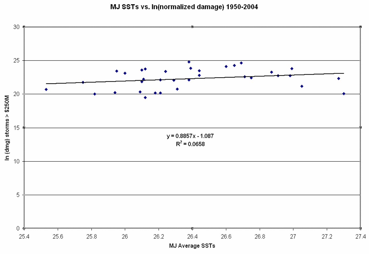
By removing 2005 the r^2 is cut in half and the p value goes up to 0.14, which is not statistically significant! So the results presented by Elsner are entirely a function of 2005, which was indeed an extreme year for both SSTs and damage. The question of whether 2005 is like seasons to come is a fair question, but I submit that the answer cannot be found in the historical data on SSTs and damage, not matter how one parses the data. Consider that if one adds 2006 to the results (damage = $250M, MJ SSTs = 26.88) the r^2 of the linear regression drops to 0.08, and the p value is 0.08, just outside statistical significance.
In short, there are a lot of ways to analyze data, and Elsner and colleagues approach is interesting. But in my view it does not provide much support for the hypothesis that SSTs are a useful or accurate predictor of damage. Anytime you have to remove 70% of the data to find a marginal (at best) relationship, it tells you that whatever relationship might exist cannot be that strong.
To underscore my perspective – future increases in Atlantic SSTs may indeed be accompanied by increases in normalized damages, but it is very difficult to accept this hypothesis based on the historical record of damage and SSTs, no matter how it is parsed. Thanks again to Jim for his continued involvement in these discussions.
October 25th, 2006 at 10:14 am
In case anyone wants the data used in this post:
year–damage (@gt $250M per storm)–MJ SSTs—ln(dmg)
2006 $250,000,000 26.88 19.33697148
2005 107,350,000,000 27.62 25.39936036
2004 48,985,385,716 26.69 24.61478784
2003 3,966,169,543 26.38 22.10106662
2002 1,055,578,444 26.31 20.77735474
1999 7,930,494,729 26.44 22.79398126
1998 4,937,282,449 27.27 22.32008091
1996 6,313,192,709 26.71 22.56590736
1995 7,444,021,043 26.91 22.730677
1992 57,663,865,630 26.38 24.77789657
1991 3,044,037,453 26.1 21.83645058
1989 15,322,273,457 25.95 23.45257339
1985 10,822,277,643 26 23.10487259
1984 285,333,505 26.12 19.46916925
1983 7,469,100,008 26.98 22.73404035
1980 1,602,040,183 27.05 21.19454377
1979 12,533,467,223 26.87 23.25166828
1976 486,444,597 25.82 20.00263357
1975 2,791,286,883 25.75 21.74976857
1974 970,296,296 25.53 20.69311204
1972 17,540,611,499 26.1 23.58778469
1971 593,886,695 25.94 20.20219911
1970 5,627,670,656 26.75 22.45096146
1969 21,225,180,492 26.99 23.77845407
1968 592,857,495 26.21 20.20046462
1967 4,016,468,362 26.21 22.11366884
1965 20,710,396,948 26.12 23.75390168
1964 15,675,871,032 26.44 23.47538849
1961 14,209,129,737 26.24 23.37715053
1960 29,619,654,069 26.6 24.11170397
1959 691,173,599 26.09 20.35390158
1958 509,818,712 27.3 20.04956575
1957 3,764,307,219 26.29 22.04882968
1956 577,494,764 26.18 20.17420993
1955 23,274,260,349 26.39 23.87061388
1954 35,671,450,726 26.65 24.29761651
1950 4,408,121,956 26.11 22.20671458
October 25th, 2006 at 2:39 pm
What percentage of the total damages was contained in those 70% of the data points that you removed?
October 25th, 2006 at 3:13 pm
LL- About 5%. 80-85% of the damage occurs with storms of category 3 or higher strength. The importance of the removed data is that is removes from the dataset years with high SSTs but low damage, like 1993, 1994, 1997, 2000, 2001, etc.
Of course, as shown in the post the relationship does not hold through 2006, even with the limited data.
October 25th, 2006 at 3:50 pm
Roger,
Please let me put this first: I’m an engineer, neither a meteorologist nor a mathematican or statistician but climate science has for years become a field of attention for me. For different reasons in the field, I am (and will probably remain) a ’soft climate sceptic’.
Nevertheless I am an engineer by heart.
Provided that the normalized loss figures and SSTs are rather correct I must say that there ist evidence that higher SSTs are prone to cause higher storm losses. The confidence level might actually not reach the usual academical level – however if I were in any business like Munich Re it would be foolish to think and act otherwise. After all 9 true out of 10 isn’t that bad a guess in business…
October 25th, 2006 at 5:24 pm
Wolfgang-
Thanks very much for your input. I certainly agree 100% with your view of statistical significance. But in this case recognize also that the question that is answered by Elsner’s work (Jagger et al.) is predicated on a conditional — experiencing storms of $250M or more within the season. If knowing when seasons are likely to be benign is important, then one would’t want to throw out years with little damage even though SSTs are high. This year is a good example of why that matters.
Because of this the graph does NOT answer the question — what happens to damages if SSTs increase?
SSTs are not a reliable predictor of damages. Have a look again at this graph:
http://sciencepolicy.colorado.edu/prometheus/archives/climate_change/000963what_does_the_histor.html#comments
Thanks!
October 25th, 2006 at 7:43 pm
The coefficients on the linear terms in the regressions are too hard to read. Also, what are their standard errors and p-values?
October 25th, 2006 at 8:35 pm
Never mind. I did the regression analysis myself. Using all your data I get:
y = -4.1096 + 0.9986x
…….. (0.78)…….(0.08)
…….. [33.9]…….[0.12]
Adjusted R^2 = 0.06
The coefficient for SST is nonsignificant at p<.10. I’d be hard-pressed to argue that there was anything going on here.
I ma catching up with this thread late, but it seems to me that SST could still predict damages, but average SST doesn’t. The problem is that if we looked hard enough we could always find some version of SST that would “do the job.”
I’m a humble country economist, not a climatologist. But that means I start from the theoretical postulate before applying statistics to data. Is there such a postulate lurking here, or is this a case of a conclusion hunting for supporting data?
October 26th, 2006 at 5:22 am
Hi Roger,
You were wrong about your data analysis (see my comment under Part 3 post of this topic) and you are wrong about our work.
At issue is the fractional change in hurricane potential destruction for the fraction of hurricanes hitting our coast that is related to Atlantic SST. A regression analysis of the log of annual damage total on SST simply does not get the job done as the analysis conflates number of loss events with loss amounts. Instead, and I repeat for the 3rd time, it is much better to model the number of loss events separately from the magnitude of losses. This is exactly what we do in Jagger et al. (2007). In this way we keep all the data (even years with no hurricane damage) and it answers the question–what happens to damages if SSTs increase. Conditional on the historical data and our model, increasing SSTs will not influence the number of loss events but they will influence the magnitude of the loss given an event.
For a more detailed and technical discussion of why you are wrong about our work jump over to our blog http://hurricaneclimate.blogspot.com/
Best,
Jim
October 26th, 2006 at 8:49 am
Jim-
Thanks. I accept the value of a “random sum” approach. But lets be clear, the point is to deconvolve a relationship. I don’t think that the intensity component of your “random sum” model is stable or shows a strong relationship. This doesn’t give me much faith in your overall model, much less making an overall argument about SSTs versus damage, for which I assert that the simple relationship I discussed in part 1 is indeed relevant.
We can of course agree to disagee and let readers decide which arguments they find compelling. I have posted another entry on this and highlighted your blog.
Thanks!
October 26th, 2006 at 9:55 am
Richard-
Thanks for your comments. You write, “Is there such a postulate lurking here, or is this a case of a conclusion hunting for supporting data?”
I am no climatologist, but I have asked Jim about the basis for expecting MJ SSTs to be correlated with damages, but not ASO SSTs, when hurricanes form, strike, and cause damage.
Thanks!
October 26th, 2006 at 1:49 pm
Roger,
I computed the r2 statistic for a linear fit to each of the 33 element subsets of your data obtained by omitting each of the years in turn.
Interestingly, knocking out 1958 increases the r2 to 0.1544 even better than omitting 2006 (0.1309). Omitting 2005 gives an r2 of 0.0323, but most values are between 0.06 and 0.09. The mean r2, although I’m not at all sure that it means anything, is 0.0857.
The values follow:
Year Damage MJ LN(Damage) r2 omitting year
2006 $250,000,000 26.88 19.33697148 0.1309
2005 107,350,000,000 27.62 25.39936036 0.0323
2004 48,985,385,716 26.69 24.61478784 0.0779
2003 3,966,169,543 26.38 22.10106662 0.0846
2002 1,055,578,444 26.31 20.77735474 0.0827
1999 7,930,494,729 26.44 22.79398126 0.085
1998 4,937,282,449 27.27 22.32008091 0.0925
1996 6,313,192,709 26.71 22.56590736 0.0841
1995 7,444,021,043 26.91 22.730677 0.0829
1992 57,663,865,630 26.38 24.77789657 0.0946
1991 3,044,037,453 26.1 21.83645058 0.0828
1989 15,322,273,457 25.95 23.45257339 0.1023
1985 10,822,277,643 26 23.10487259 0.0959
1984 285,333,505 26.12 19.46916925 0.0733
1983 7,469,100,008 26.98 22.73404035 0.083
1980 1,602,040,183 27.05 21.19454377 0.1064
1979 12,533,467,223 26.87 23.25166828 0.0787
1976 486,444,597 25.82 20.00263357 0.0631
1975 2,791,286,883 25.75 21.74976857 0.082
1974 970,296,296 25.53 20.69311204 0.0644
1972 17,540,611,499 26.1 23.58778469 0.098
1971 593,886,695 25.94 20.20219911 0.0688
1970 5,627,670,656 26.75 22.45096146 0.0848
1969 21,225,180,492 26.99 23.77845407 0.0725
1968 592,857,495 26.21 20.20046462 0.0788
1967 4,016,468,362 26.21 22.11366884 0.0845
1965 20,710,396,948 26.12 23.75390168 0.099
1964 15,675,871,032 26.44 23.47538849 0.0862
1961 14,209,129,737 26.24 23.37715053 0.0913
1960 29,619,654,069 26.6 24.11170397 0.0819
1959 691,173,599 26.09 20.35390158 0.0747
1958 509,818,712 27.3 20.04956575 0.1544
1957 3,764,307,219 26.29 22.04882968 0.0843
1956 577,494,764 26.18 20.17420993 0.0775
1955 23,274,260,349 26.39 23.87061388 0.089
1954 35,671,450,726 26.65 24.29761651 0.0799
1950 4,408,121,956 26.11 22.20671458 0.0854
October 26th, 2006 at 5:45 pm
D.F.- Interesting, thanks …
October 26th, 2006 at 8:38 pm
I’m not sure what to make of the various statistical analyses. A model that explains about 10% of the variance is of course missing 90% of it. I’d rather focus on trying to explain more of that 90% than refine whether the model can be fine tuned to get 10% +/- 1% instead of 10%+/- 4%. With 90% of the variance unexplained, we cannot discern an unbiased model that happens to have a lot of noise from a model that’s more lucky than accurate.
I will hazard (!) a guess that most of that 90% is explained, if at all, by economic and political factors — not climate. Economic damages from Katrina appear to have resulted mostly from ancillary phenomena, such as the peculiar political cultures of the U.S Congress (earmarking in lieu of benefit-cost analysis to allocate ACE resources) and New Orleans (’nuff said).
I also want to admit that if a MJ SST and an ASO SST both came to the door, I’d just pay for the pizza. If higher SSTs cause more intense storms (my boneheaded economist’s interpretation of Elsner’s posts), averaging over time and space (whether MJ or ASO) seems to me to be an inefficient way to discover it. If I were July, I’d sue for discrimination.
October 26th, 2006 at 8:43 pm
I;m not sure what to make of the various statistical analyses. A model that explains about 10% of the variance is of course missing 90% of it. I’d rather focus on trying to explain more of that 90% than refine whether the model can be fine tuned to get 10% +/- 1% instead of 10%+/- 4%. With 90% of the variance unexplained, we cannot discern an unbiased model that happens to have a lot of noise from a model that’s more lucky than accurate.
I will hazard (!) a guess that most of that 90% is explained, if at all, by economic and political factors — not climate. Economic damages from Katrina appear to have resulted mostly from ancillary phenomena, such as the peculiar political cultures of the U.S Congress (earmarking in lieu of benefit-cost analysis to allocate ACE resources) and New Orleans (’nuff said).
I also want to admit that if a MJ SST and an ASO SST both came to the door, I’d just pay for the pizza. There are a lot more policy levers iurking in the unexplained variance.