Recap: Atlantic SSTs and U.S. Hurricane Damages
October 27th, 2006Posted by: Roger Pielke, Jr.
We’ve had an interesting discussion this week on the historical relationship of Atlantic sea surface temperatures and U.S. hurricane damage. I began by asking:
What Does the Historical Relationship of Atlantic Sea Surface Temperature and U.S. Hurricane Damage Portend for the Future?
This post provides a recap of the week’s discussion.
I answered the initial question with two perspectives, one that I prepared and one by Munich Re’s Eberhard Faust. The conversation was quickly joined by noted hurricane expert Jim Elsner from Florida State, who claimed that his preferred approach definitively resolved this question. Jim and I have had a lengthy exchange this week in the comments, including an effort on my part to replicate part of his analysis, successful in the end, but with a mistake along the way. Thanks to Jim for helping make this replication successful
Even with the lengthy exchange, I remain confused about what Elsner is arguing. He has claimed that the signal of SST couldn’t be seen using all historical damage data in a simple regression because of the effects of the North Atlantic Oscillation (NAO). Here is how Jim described it:
Sometimes when the Atlantic is warm and hurricanes are strong, the steering flow keeps them from reaching the US and the steering during the season can be predicted to some degree by preseason values of the NAO; thus a simple regression of annual loss on SST is inadequate for understanding the relationship between loss and SST.
This last phrase – “a simple regression of annual loss on SST is inadequate for understanding the relationship between loss and SST.” – seems completely consistent with the focus of my original post in which I asserted that a relationship between SSTs and damage “may materialize in the future, but one cannot use the past to project such a relationship, it must be based on some other considerations.” Elsner, it would seem, agreed that “other considerations” (e.g., like the NAO) actually matter for the ability to identify a signal. But Jim would have none of this potential agreement. He later made what appears to be the opposite argument, that the future influence of SST on damages would be identifiable independent of the NAO, explaining that “The correlation between tropical SST and NAO is small.” Either the NAO masks or does not mask a SST signal, it cannot be both — hence my confusion.
Lost in these very fine points about very marginal statistical relationships is the fact that Jim and I are pretty close in our views, no matter how aggressively he objects to each point that I make. He writes of his answer to my original question about what the past relationship of SSTs and damage tells us about the future:
If all we know are SST and damages from history, then I would assign a personal probability of 60-70% that over the next 100 years the warm SST years will, on average, have greater annual loss totals compared to the cold SST years.
If I were to modify Jim’s statement to more accurately reflect my own perspective, I’d simply change 60-70% to 50%, which in my view is not a particularly big difference. I therefore don’t see our views as being particularly far off from one another (though I am sure that Jim would strongly disagree;-).
I’ll close by referring the reader back to the first post presented in this discussion, and the two graphs that I presented.
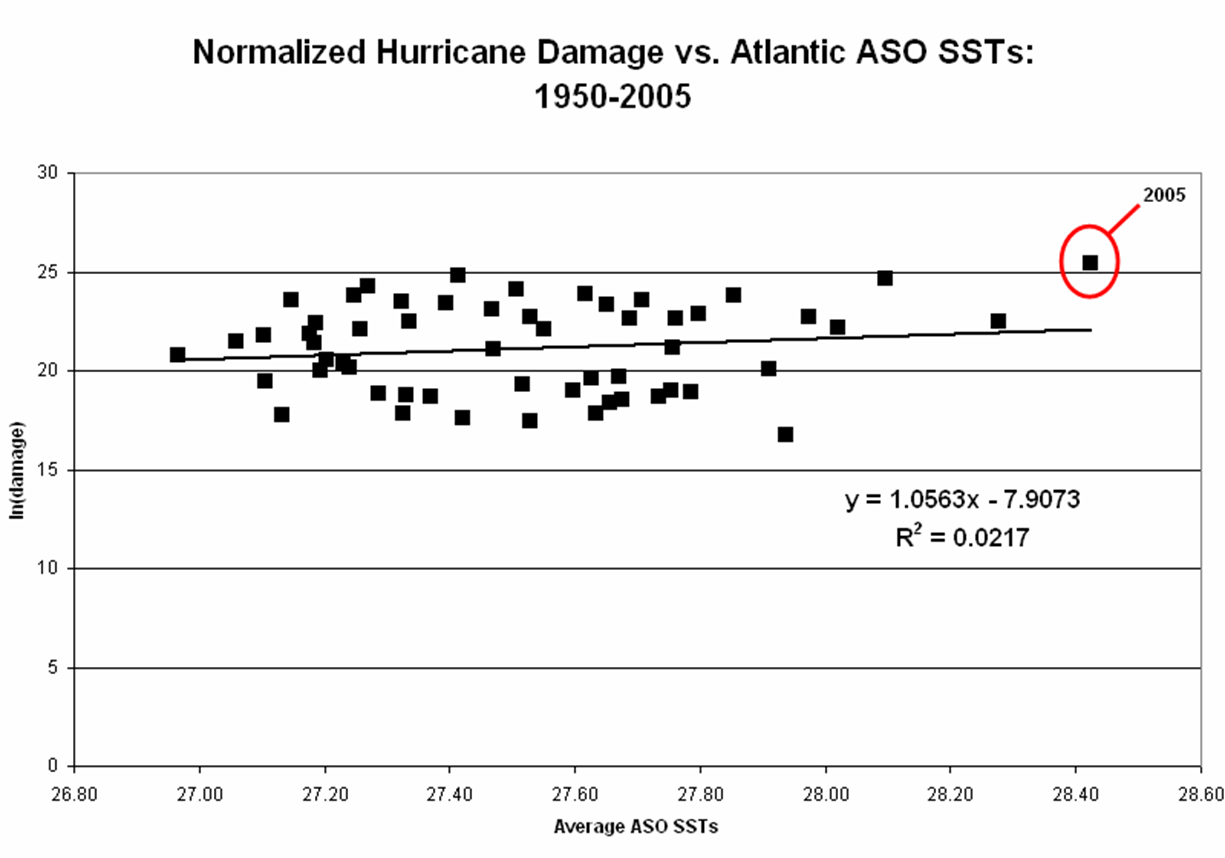
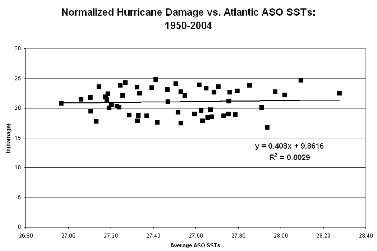
To provide my answer to the question posted in Part 1 that kicked off this discussion. If all you know is SSTs and U.S. damage from the historical record — that is, the data shown in these graphs – then you have no statistical basis for saying what will happen in the future if SSTs increase. Faust suggests that by looking at a subset of the data a stronger relationship can be seen. Elsner suggests that by introducing other climate variables than those presented here and distinguishing intensity from frequency a stronger relationship can be seen. Both Faust’s and Elnser’s points are fairly made. For reasons that you’ll find in the discussion this past week, I find that accepting their arguments at face value (i.e., setting aside the appropriateness of looking at a limited subset of data or the stability of relationships over time) leads to only marginal relationships (at best) whose existence are dependent upon the data of 2005. Sometimes the simplest analysis tells the whole story.
Future increases in Atlantic SSTs may indeed be accompanied by larger amounts of U.S. hurricane damage. But I find little basis for this conclusion in the overall historical record of SSTs and damage. Others disagree. I respect their views, but remain unconvinced by their analyses. If nothing else this exercise has been a wonderful example of the diversity of the scientific enterprise, and how seemingly simple questions are subject to a range of legitimate perspectives. The good news is that effective hurricane policies need not await consensus on this issue!
[Thanks to those of you who emailed ideas and comments!]
October 27th, 2006 at 8:22 am
Jim-
Your paper states:
“The models and data are available on our web site (http://garnet.fsu.edu/jelsner/www/)”
I cannot locate either the data or the models on your WWW site, can you provide a direct link?
Thanks!!
October 27th, 2006 at 11:23 am
Hi Roger,
“Future increases in Atlantic SSTs may indeed be accompanied by larger amounts of U.S. hurricane damage.”
Even this possibility is not necessarily relevant to a policymaker. If I download your data on the adjusted damage from hurricanes for the years 1950 to 2006, I get an arithmetic mean value of $13.5 billion.
Further, your research has pointed very clearly to the conclusion that adjusting to future years will bring even higher damage levels, because the damage is increasing much faster than inflation (due to more increasingly wealthy people moving nearer to the coast).
But let’s assume that the values stay the same, and the next 56 years would bring an annual average of $13.5 billion WITHOUT any global warming. The question STILL is, “What will it be WITH global warming?”
If the answer is “higher; approximately $13.7 billion per year”…well, that’s trivial.
It’s only if the answer is something like, “higher…$27 billion per year” (i.e., twice as much) that it MIGHT make a difference from a policy standpoint.
“The good news is that effective hurricane policies need not await consensus on this issue!”
Yes, let’s deploy the water tube hurricane storm surge protection system, ASAP!
P.S. And when we see how well that system works, let’s talk about how to go about reducing hurricane strength…thus reducing wind and inland flooding damage.
October 27th, 2006 at 12:18 pm
Roger,
Saying, as I have, that “a simple regression of annual loss on SST is inadequate for understanding the relationship between loss and SST” is quite different than what you are saying with “signal of SST couldn’t be seen using all historical data”. It is not appropriate to use a regression of the log of annual losses on SST as a basis for addressing this relationship. Can you tell me what 10% of the variability in log annual losses means in terms of actual losses?
I never claimed my “approach definitively resolved this question”, only that it is a better tool to address the issue of a potential relationship between losses and SST than your approach or Faust’s approach. Allow me an analogy. If the question is which tool is best for securing a leg to a table using a screw with the choices being a hammer or an awl, then the answer would be neither; it is best to use a screw driver. You can argue about the quality of the results obtained with the screw driver, but it remains the better tool to use and someone who knows how to use a screw driver is better qualified to judge the quality of the work.
You continue to compare apples with oranges. As a sensitivity test to our more complex conditional probability model, we regress the log of PER EVENT losses on preseason SST. We find a significant relationship (p=0.0086). You use different data, a shorter record, and regress the log of TOTAL ANNUAL losses on seasonal SST. As a criticism of my results, your analysis and results are only marginally relevant.
As an aside. Why have 6 different entries on a single topic?
The book is due out next year. The models and data are available with the lead author Thomas Jagger. What papers are published that show no relationship between damage and SST?
Best,
Jim
October 27th, 2006 at 12:52 pm
Jim-
Thanks.
Analogies about screwdrivers and tables are great. But why not simply just share your data and methods? The paper does not provide the data, nor does your WWW site as the paper claims it does. I would have a far better chance of understanding your complaints if you simply shared the dataset. What is the problem with that?
For instance, your dataset would be important for understanding your claim of the significance of treating storms on an annual basis versus a per storm basis. I used annual values of storms with >$250M in damage and generated the _exact same results_ as you reported 1950-2005. This is not surprising, and I doubt explains anything. But I can’t know because you haven’t simply shared your data — you’ve just made assertions.
When you are ready to share your data I’ll be happy to revisit your analysis. I’ve shared my data here, and that helped you to understand what I was doing an indeed to identify a mistake. I shared my data in good faith, how about you return the favor?
Thanks!
October 27th, 2006 at 3:20 pm
Could someone please direct me to the numeric data underlying the two charts (Normalized Hurricane Damage v. Atlantic SST) in this post.
Thanks,
Don
October 27th, 2006 at 3:55 pm
Donald- Here you go:
year–ASO SST–normalized damage–ln(dmg)
1950 27.19 $5,529,320,501 22.43333077
1951 27.67 $358,069,353 19.69623725
1952 27.68 $114,732,781 18.55811634
1953 27.63 $55,787,059 17.83705248
1954 27.27 $35,671,450,726 24.29761651
1955 27.62 $23,274,260,349 23.87061388
1956 27.24 $577,494,764 20.17420993
1957 27.55 $3,841,822,355 22.06921266
1958 27.91 $509,818,712 20.04956575
1959 27.20 $858,779,107 20.5710223
1960 27.51 $29,970,493,213 24.12347918
1961 27.39 $14,468,733,186 23.39525583
1962 27.66 $92,192,732 18.33939186
1963 27.52 $246,291,959 19.32202822
1964 27.32 $15,693,459,358 23.47650986
1965 27.25 $21,261,254,041 23.78015219
1966 27.63 $336,552,296 19.63426411
1967 27.26 $4,016,468,362 22.11366884
1968 27.23 $657,263,225 20.30359514
1969 27.85 $21,225,180,492 23.77845407
1970 27.34 $5,627,670,656 22.45096146
1971 27.06 $2,083,668,167 21.45739572
1972 27.15 $17,579,304,340 23.58998816
1973 27.33 $145,454,945 18.79537694
1974 26.97 $1,073,783,964 20.79445466
1975 27.10 $2,791,286,883 21.74976857
1976 27.19 $486,444,597 20.00263357
1977 27.33 $53,776,992 17.80035628
1978 27.29 $145,903,706 18.79845741
1979 27.65 $14,096,216,718 23.36917228
1980 27.76 $1,602,040,183 21.19454377
1981 27.60 $171,359,510 18.95927431
1982 27.42 $43,148,911 17.58016773
1983 27.53 $7,469,100,008 22.73404035
1984 27.11 $289,628,417 19.48410934
1985 27.47 $11,068,101,797 23.1273331
1986 27.13 $50,026,988 17.72807318
1987 27.94 $19,011,511 16.76055519
1988 27.75 $172,912,773 18.96829783
1989 27.71 $16,770,856,131 23.54290846
1990 27.73 $126,787,371 18.658022
1991 27.18 $3,044,037,453 21.83645058
1992 27.41 $57,663,865,630 24.77789657
1993 27.37 $126,479,971 18.65559452
1994 27.18 $1,938,752,062 21.38531034
1995 27.97 $7,501,957,030 22.73842976
1996 27.69 $6,537,460,457 22.60081462
1997 27.79 $163,560,186 18.91269159
1998 28.28 $6,021,601,438 22.51861908
1999 27.80 $8,277,977,785 22.83686455
2000 27.53 $36,525,742 17.41352783
2001 27.76 $6,970,450,131 22.66494564
2002 27.47 $1,491,060,293 21.12275331
2003 28.02 $4,212,081,525 22.16122279
2004 28.10 $49,130,243,738 24.61774064
2005 28.42 $107,350,000,000 25.39936036
October 27th, 2006 at 6:18 pm
Roger,
I would like to continue this discussion with you in Greece next spring at our Summit on Hurricanes and Climate Change (http://www.aegeanconferences.org/). Please email me or give me a call if you are interested in attending.
Best,
Jim
October 27th, 2006 at 9:32 pm
Jim- Thanks kindly for the gracious invitation. I’ll give a call next week. Thanks!
October 31st, 2006 at 5:50 am
Perhaps I missed this in the deluge of comments. Have the damage estimates been validated as unbiased? They are disturbingly precise, down to the nearest dollar (!) in many cases.
Along those lines, regression analysis assumes that the data are measured accurately. Given the marginal size of the estimated effect — in all of the models discussed here — measurement error on the damage function could be greater than the magnitude of the effect being measured.
A final theoretical question, which I think I raised earlier but don’t recall a persuasive answer. It’s not obvious to me what we should want to measure when measuring economic damages from hurricanes. I’m uncomfortable with both insured and uninsured losses as appropriate theoretical measures; that distinction has more to do with the idiosyncracies of the market and the normal gambling that both insurers and insureds willingly and knowingly undertake. Because of that gambling, insurance coverage in year n+1 is correlated with losses in year n. I know this matters but I haven’t a clue what to do with it. We shouldn’t ignore this question because losses will depend on the proportion of assets under coverage. Finally, any jurisdiction that by regulation achieves 100% coverage experiences disastrous adverse selection and moral hazard problems. (Cf. the federal flood insurance program.)
Is the choice of insured vs. uninsured damages a debate over which lamp post to look under?
A colleague in New Jersey considering a move to the Florida coast watched the “Hardball” debate between the R and D candidates for governor, whose names I have forgotten if I ever knew them. He was particularly interested in the question how each candidate proposed to deal with the “insurance problem” there, which I gather can be shorthanded as “people on the coast don’t want to pay the full cost of living there.”
According to my colleague, the D candidate’s solution is to use state regulation to mandate lower insurance premiums and higher coverage. Such a policy would shift cost to inland residents. Because on average they are much less wealthy, this policy transfers wealth from rich to poor (i.e., a “reverse Robin Hood”). The R candidate’s solution is to federalize the coastal insurance market. Such a policy would shift cost to residents of non-hurricane vulnerable coastal counties or federal taxpayers generally. That would transfer wealth to those who live in hurricane-vulnerable areas, but it’s not clear whether it’s also a reverse Robin Hood. (The residents of Pebble Beach are not obviously economically disadvantaged compared to the residents of Palm Beach.)
Choosing between these proposed policies is not easy. Florida voters as a whole should prefer the R’s policy because it externalizes cost out of state. The problem is it’s virtually certain never to be enacted. The D’s policy is implementable at the state level, but of course it’s highly divisive within the state once its wealth transfer effects are made transparent. But either policy would distort individual behavior in ways that increase future losses from hurricanes by a much greater amount than the 10% or so of variance we are debating.
October 31st, 2006 at 7:59 am
Richard- Thanks for these excellent comments. We will be posting up a submitted paper along with data later this week which discusses the normalization methodology and associated uncertainties. I’d be happy to take up the discussion then, as the paper does go someway I think to answering your questions.
Thanks!
November 2nd, 2006 at 1:42 pm
As an engineer I am having a hard time believing what I’m reading.
It seems that; (1) there are major questions about exactly how to measure the dependent quantity (damage): and (2) there has been little discussion of how the chosen independent quantity (SST) relates to the actual physical processes that lead to damage. By the latter I mean primarily how does SST determine that the path of the storm includes structures/objects/materials that can undergo damage. Additionally, the amount of the physcial damage is primarily a function of the quality and quantity of the structures/objects/materials that are in the path. And this leads us back to (1) above.
If a paper on this subject was sent to me for review for publication in an engineering journal, and the authors did not address such fundamental issues, I would reject it.
A metric which does not connect cause and effect is not a valid metric.
November 16th, 2006 at 4:27 am
Roger,
I linked your new per-event normalized damages to NA-SST and tried to apply Jim’s method of seperating noise from signal using the pareto principle mentioned in his paper. For your PL05 data noise cutoff turned out to be app. 5E9 US$.
Using this subset of events no trend was appearent.
Regards,
Wolfgang
****
****
R-transcript:
> imp<-read.table(“clipboard”,header=T,sep=”;”,dec=”.”) # import data (see below) from clipboard
> hursstPL05<-imp[order(imp$PL05,decreasing=T,na.last=T),-7] # rank sort REM we don’t need CL05 data here
> names(hursstPL05)
[1] “Yr” “MonthStart” “DayStart” “StormName” “BaseDamage” “PL05″ “NATLSST”
> hursstPL05$cPL05<-cumsum(hursstPL05$PL05) #calc cumulated sum of ranked PL05 normalized damages
> hursstPL05$cPL05<-hursstPL05$cPL05/hursstPL05$cPL05[nrow(hursstPL05)] #make cumulated sum of PL05 relative to total losses (which is the last row’s cPL05 value)
> hursstPL05$Rank <- 1-(1:nrow(hursstPL05)/nrow(hursstPL05)) # make rank relative REM 1-(…) is for convenience, pareto point is now close to 0.8/0.8
> plot(hursstPL05$Rank,hursstPL05$cPL05) # this looks very much like Jim’s results (keep in mind x axis has been mirrored)
> plot(hursstPL05$PL05,hursstPL05$cPL05-hursstPL05$Rank);grid() # since rank and cumsum are now both relative we look for pareto cutoff point (x axis intercept) REM from the prev plot, this is where pareto curve intercepts with line y=x, so we try to estimate y-x=0
> plot(hursstPL05$PL05,hursstPL05$cPL05-hursstPL05$Rank,xlim=c(0,1E10),ylim=c(-0.1,0.1));grid() # magnify region of interception for a better estimate
> locator() # let’s pick the interception by pointing and clicking (y=0) for convenience
$x
[1] 5334434352
$y
[1] 0.0002515137
> # this is close enough – 53E8 US$ becomes random damage cutoff
> plot(hursstPL05$NATLSST,log10(hursstPL05$PL05));grid() # now let’s plot log(PL05) over SST
> cutoffdamage<-53E8 # taken from locator above
> abline(h=log10(cutoffdamage),col=”grey”) # show cutoff damage line – sorry not many signal points there
> hursstPL05.lma<-lm(log10(PL05)~NATLSST,data=hursstPL05) # declare the overall model w/o cutoffs
> abline(hursstPL05.lma) # draw it
> summary(hursstPL05.lma) # show me the model data
Call:
lm(formula = log10(PL05) ~ NATLSST, data = hursstPL05)
Residuals:
Min 1Q Median 3Q Max
-3.5179 -0.7580 -0.0271 0.8604 2.2249
Coefficients:
Estimate Std. Error t value Pr(>|t|)
(Intercept) 3.1588 4.3086 0.733 0.465
NATLSST 0.1954 0.1560 1.253 0.212
Residual standard error: 1.109 on 146 degrees of freedom
Multiple R-Squared: 0.01063, Adjusted R-squared: 0.003855
F-statistic: 1.569 on 1 and 146 DF, p-value: 0.2124
> hursstPL05.lmc<-lm(log10(PL05)~NATLSST,data=subset(hursstPL05,log10(PL05)>log10(53E8))) # now for the signal subset using >53E8 US$ cutoff
> abline(hursstPL05.lmc,col=”red”) # draw it
> summary(hursstPL05.lmc) # show me the model data
Call:
lm(formula = log10(PL05) ~ NATLSST, data = subset(hursstPL05,
log10(PL05) > log10(5.3e+09)))
Residuals:
Min 1Q Median 3Q Max
-0.3618 -0.2485 0.0368 0.1414 0.7611
Coefficients:
Estimate Std. Error t value Pr(>|t|)
(Intercept) 9.33716 2.62342 3.559 0.00167 **
NATLSST 0.02847 0.09445 0.301 0.76581
—
Signif. codes: 0 ‘***’ 0.001 ‘**’ 0.01 ‘*’ 0.05 ‘.’ 0.1 ‘ ‘ 1
Residual standard error: 0.2971 on 23 degrees of freedom
Multiple R-Squared: 0.003934, Adjusted R-squared: -0.03937
F-statistic: 0.09085 on 1 and 23 DF, p-value: 0.7658
****
Data sources:
Normalized damages:
http://sciencepolicy.colorado.edu/publications/special/normalized_hurricane_damages.html
Link hurricane year+name to storm start date:
http://www.climateaudit.org/data/hurricane/unisys/Track.ATL.txt
Monthly NA-SST:
http://www.cpc.noaa.gov/data/indices/sstoi.atl.indices
Data:
Yr;MonthStart;DayStart;StormName;BaseDamage;PL05;CL05;NATLSST
1950;9;1;Easy;3300000;1121198545.08702;972672385.007333;27.78
1950;10;13;King;28000000;4408121956.38413;3725252507.43757;27.69
1951;9;28;How;2000000;358069352.97984;328708795.322242;27.97
1952;8;18;Able;2800000;114732781.485231;158056794.917681;27.65
1953;8;11;Barbara;1000000;43764416.0158102;76617081.0355628;27.68
1953;9;23;Florence;200000;12022642.7780337;14316188.3703613;27.94
1954;8;25;Carol;460000000;16133671673.3372;15084813860.1831;27.25
1954;9;2;Edna;40000000;3024742035.74783;1669025614.16583;27.68
1954;10;5;Hazel;281000000;16513037016.9668;23245567610.428;27.36
1955;8;3;Connie;40000000;2321631096.31438;3809221512.46724;27.64
1955;8;7;Diane;800000000;17212609735.9547;17830947063.839;27.64
1955;9;10;Ione;88000000;3740019516.49593;6004736906.56358;28.08
1956;9;21;Flossy;25000000;577494763.566377;711117719.385467;27.63
1957;6;25;Audrey;150000000;3764307219.24643;4122645630.76675;26.61
1957;9;16;Esther;2000000;77515135.6201929;88441730.0662904;28.05
1958;9;21;Helene;11200000;509818712.22738;643883845.33683;28.11
1959;5;28;Arlene;1000000;26834452.4134174;31975141.8960604;25.83
1959;7;23;Debra;7000000;317622133.00818;287583193.32736;26.66
1959;9;20;Gracie;14000000;373551466.137319;509799371.738114;27.75
1959;6;18;NOTNAMED;2000000;140771055.072183;132753509.251097;26.34
1960;7;28;Brenda;5000000;184889923.928569;274187875.486212;27.12
1960;8;29;Donna;300000000;26817811904.9043;28920699578.6421;27.53
1960;8;29;Donna;87000000;2801842164.31962;2977933407.36724;27.53
1960;9;14;Ethel;1000000;29098891.2744484;32844899.5847996;27.87
1960;6;22;NOTNAMED;4000000;136850328.600666;139399585.618997;26.91
1961;9;3;Carla;400000000;14209129736.954;13466621200.0789;27.76
1961;9;10;Esther;6000000;259603449.376759;183786233.664288;27.76
1962;8;26;Alma;1000000;77570243.5161737;81268979.0598545;27.69
1962;9;29;Daisy;1000000;14622488.5659346;18733899.3549728;27.94
1963;9;16;Cindy;13000000;246291959.184626;242741064.476109;27.94
1964;8;5;Abby;1000000;17588326.5935661;18247717.797249;27.44
1964;8;20;Cleo;128000000;5173116167.57032;4653166630.79856;27.44
1964;8;28;Dora;250000000;7682229901.66649;6577589727.86072;27.44
1964;9;28;Hilda;125000000;2186382636.85263;2592839590.84212;27.59
1964;10;8;Isbell;10000000;634142325.701495;624127559.148902;27.57
1965;8;27;Betsy;142000000;2853986824.84002;4013938352.4303;27.16
1965;8;27;Betsy;1278000000;17856410123.1602;19030722651.0489;27.16
1965;9;24;Debbie;25000000;550857093.310467;618312616.803641;27.74
1966;6;4;Alma;10000000;243643316.823062;251656976.575758;26.9
1966;9;21;Inez;5000000;92908979.295204;130663799.98004;28.02
1967;9;5;Beulah;200000000;4016468362.23148;4047098432.03278;27.74
1968;6;1;Abby;1000000;31949630.694152;30828136.3170355;26.36
1968;6;22;Candy;3000000;32456099.4118217;36750158.6021393;26.36
1968;10;13;Gladys;7000000;592857495.099422;495114444.590688;27.72
1969;8;14;Camille;1421000000;21225180491.8357;23957867600.018;27.82
1970;7;31;Celia;454000000;5627670656.11602;5719215718.16093;26.9
1971;8;20;Doria;147000000;1334299277.62303;1307086502.41289;27.1
1971;9;5;Edith;25000000;259842605.917541;281485526.148339;27.58
1971;9;3;Fern;30000000;334044089.23212;342638045.106185;27.58
1971;9;6;Ginger;10000000;155482194.461511;214628140.653225;27.58
1972;6;14;Agnes;31000000;348605988.334489;411000085.922878;26.34
1972;6;14;Agnes;1969000000;17192005511.1422;18027963064.6195;26.34
1972;8;29;Carrie;2000000;38692840.2976145;35153384.7629863;27.17
1973;9;1;Delia;18000000;145454945.455995;151640798.813589;27.74
1974;8;29;Carmen;150000000;970296296.479568;1103059329.2921;26.98
1974;10;4;SUBTROP4;10000000;103487667.925113;96054210.188275;27.3
1975;9;13;Eloise;490000000;2791286883.13172;2834851643.30456;27.44
1976;8;6;Belle;100000000;486444597.249696;480358141.453008;27.28
1977;9;3;Babe;10000000;53776992.1291894;60998836.6104761;27.75
1978;7;30;Amelia;20000000;145903705.971742;156202197.451051;26.8
1979;7;9;Bob;20000000;55497618.0057935;66073062.6813304;27.25
1979;7;15;Claudette;400000000;1472033641.13539;1578948268.8432;27.25
1979;8;25;David;320000000;2265907697.29244;2193891625.55571;27.67
1979;8;30;Elena;10000000;35218235.6839325;39149979.5112807;27.67
1979;8;29;Frederic;2300000000;10267559525.8002;11537923782.9407;27.67
1980;7;31;Allen;300000000;1602040183.30964;1743702284.88263;27.24
1981;8;7;Dennis;25000000;171359510.015338;160414409.951321;27.61
1982;9;9;Chris;2000000;5712609.37392955;6082318.74386322;27.82
1982;6;18;SUBTROP1;10000000;37436301.3224476;34977305.1310577;26.73
1983;8;15;Alicia;2000000000;7469100008.23059;7247139031.89662;27.56
1984;9;8;Diana;65000000;285333504.681358;309924883.982795;27.6
1984;9;25;Isadore;1000000;4294911.87141379;3782009.26582964;27.6
1985;7;21;Bob;25000000;109802229.64988;108568222.658689;27.01
1985;8;12;Danny;50000000;136021923.977223;142611996.564959;27.52
1985;8;28;Elena;1250000000;3573151699.89441;3769907745.52291;27.52
1985;9;16;Gloria;900000000;2364496011.89072;2398943773.6603;27.87
1985;10;26;Juan;1500000000;3867650060.19267;4207280862.07152;27.58
1985;11;15;Kate;300000000;1016979871.43563;1088138521.05121;27.34
1986;6;23;Bonnie;2000000;4839644.88043428;4724217.96326887;26.13
1986;8;13;Charley;15000000;45187343.0571066;49674771.5405767;27.16
1987;10;9;Floyd;1000000;2371775.26466554;2649286.39799291;28.39
1987;8;9;NOTNAMED;7000000;16639735.5750958;15795937.8411339;28.09
1988;8;8;Beryl;3000000;5868431.20953051;5796936.11869893;27.73
1988;8;21;Chris;1000000;2627965.37056287;2675388.47621617;27.73
1988;9;7;Florence;2000000;4259184.7309039;4640241.44666382;28.06
1988;9;8;Gilbert;50000000;151642640.754396;160583720.535914;28.06
1988;11;17;Keith;3000000;8514551.38873669;8102891.06578335;27.35
1989;6;24;Allison;500000000;1049664034.83642;1033461438.00434;26.38
1989;7;30;Chantal;100000000;228680309.482794;218804501.895467;27.29
1989;9;10;Hugo;7000000000;15322273456.8102;17483447130.5762;27.89
1989;10;12;Jerry;70000000;170238330.092162;164551637.940327;27.89
1990;10;9;Marco;57000000;126787371.06728;120235627.094055;28.18
1991;8;16;Bob;1500000000;3044037453.10207;3066892329.81044;27.16
1992;8;16;Andrew;25500000000;55766925398.4863;52340623757.8588;27.44
1992;8;16;Andrew;1000000000;1896940231.87161;1996613736.53536;27.44
1993;6;18;Arlene;22000000;44109986.3527193;43461800.0472994;26.7
1993;8;22;Emily;35000000;82369985.0102556;77179506.289198;27.35
1994;6;30;Alberto;500000000;1005181421.78775;1017035501.35262;26.04
1994;8;14;Beryl;73000000;148740712.164718;153918448.877874;27.29
1994;11;8;Gordon;400000000;784829927.88167;783043644.190887;27.37
1995;6;3;Allison;1700000;3214014.85809597;3245587.7819801;27.05
1995;7;28;Dean;500000;952665.685336516;924870.705451224;27.49
1995;7;31;Erin;500000000;953967722.888713;953197728.498768;27.49
1995;7;31;Erin;200000000;405628332.494382;422663718.2098;27.49
1995;8;22;Jerry;26500000;53769306.4535895;49977884.2646661;28.07
1995;9;27;Opal;3000000000;6084424987.41573;6339955773.14699;28.36
1996;7;5;Bertha;270000000;491228251.162088;520502972.952672;27.15
1996;8;23;Fran;3200000000;5821964458.21734;6168924123.88352;27.74
1996;10;4;Josephine;130000000;224267747.6416;235746491.065523;28.01
1997;7;16;Danny;100000000;163560186.413961;168484613.292749;27.38
1998;8;19;Bonnie;720000000;1163745048.09035;1214916672.09466;28.35
1998;8;21;Charley;50000000;79242707.2029009;77442127.0438009;28.35
1998;8;31;Earl;79000000;125092557.753638;126232888.654257;28.35
1998;9;8;Frances;500000000;809646688.76287;783835954.874037;28.6
1998;9;15;Georges;680000000;987880134.296214;1046295571.39035;28.6
1998;9;15;Georges;1630000000;2785657266.26725;2524834055.31156;28.6
1998;10;22;Mitch;40000000;70337036.0996478;69346466.6141704;28.46
1999;8;18;Bret;60000000;76412678.0135494;93900756.7595772;27.87
1999;8;24;Dennis;157000000;246762368.324441;248150280.969978;27.87
1999;9;7;Floyd;4500000000;6714795179.51099;6787052608.93818;28.25
1999;9;19;Harvey;15000000;24308009.6960988;24022769.1984891;28.25
1999;10;12;Irene;800000000;1215699549.51022;1178217657.93973;28.15
2000;9;14;Gordon;10000000;13867299.1421151;13574119.2734164;27.91
2000;9;15;Helene;16000000;22658442.7794139;23238835.700727;27.91
2001;6;5;Allison;5000000000;6622921397.06239;6445689806.90606;26.61
2001;8;2;Barry;30000000;39667764.8001923;40210381.7100888;27.77
2001;9;11;Gabrielle;230000000;307860968.819143;306339576.949535;28.27
2002;9;5;Fay;5000000;6091464.86053774;6065422.95383364;27.93
2002;9;8;Gustav;100000;125699.708144247;126296.31724032;27.93
2002;9;12;Hanna;20000000;24750816.8454853;24893394.5158999;27.93
2002;9;14;Isidore;330000000;398215397.267126;399319939.980315;27.93
2002;9;20;Kyle;5000000;6298469.56574654;6373619.31802296;27.93
2002;9;21;Lili;860000000;1055578444.29777;1060811848.40661;27.93
2003;6;28;Bill;30000000;34960159.9520769;35278638.9583616;26.62
2003;7;7;Claudette;180000000;210951821.349526;210140801.978706;27.3
2003;9;6;Isabel;3370000000;3966169543.4725;3989771692.97868;28.63
2004;7;31;Alex;4000000;4329688.17639211;4334942.52415457;27.44
2004;8;9;Charley;15000000000;16319033805.8813;16297047080.3953;28.2
2004;8;25;Frances;8900000000;9683982516.70226;9648997103.32787;28.2
2004;8;27;Gaston;130000000;140528333.931716;141215672.29431;28.2
2004;9;2;Ivan;14200000000;15473790997.7962;15514011620.257;28.65
2004;9;13;Jeanne;6900000000;7508578395.85992;7496264391.31465;28.65
2005;7;3;Cindy;320000000;320000000;320000000;28.06
2005;7;4;Dennis;2230000000;2230000000;2230000000;28.06
2005;8;23;Katrina;81000000000;81000000000;81000000000;28.46
2005;9;6;Ophelia;1600000000;1600000000;1600000000;28.75
2005;9;18;Rita;10000000000;10000000000;10000000000;28.75
2005;10;15;Wilma;20600000000;20600000000;20600000000;28.57